Loading EOIR Texture Maps From NASA's Earthdata

STK 12.5 introduces the capability to create your own custom reflectance, emissivity, temperature, and radiance maps to add fidelity to your EOIR analysis. There is a wealth of publicly available science data on the internet, and you can process the data for import into STK. In the examples below, you will import radiance data from an HDF4 (*.hdf) file and temperature data from an HDF5 (*.h5) file. Start by creating an account on NASA's Earthdata service. Find and select the data of your choice and review the specific documentation available from the publishers with that dataset. It is important to get the desired band measurement wavelengths, as it is a required input into STK for radiance, emissivity, and reflectivity maps. In these examples, you will use datasets MOD11A2 for land surface temperature data and VNP46A2 for night-light radiance data. Instructions are available below using HDFView and Microsoft Excel, Matlab, or Python. A running list of general notes is also available at the bottom of this document. Do you want to see this in action? Check out the AGI feature demo video on Youtube.

HDFView and Microsoft Excel

HDF4 (*.hdf) processing

1. Ensure that you have HDFView and Microsoft Excel installed on your computer.
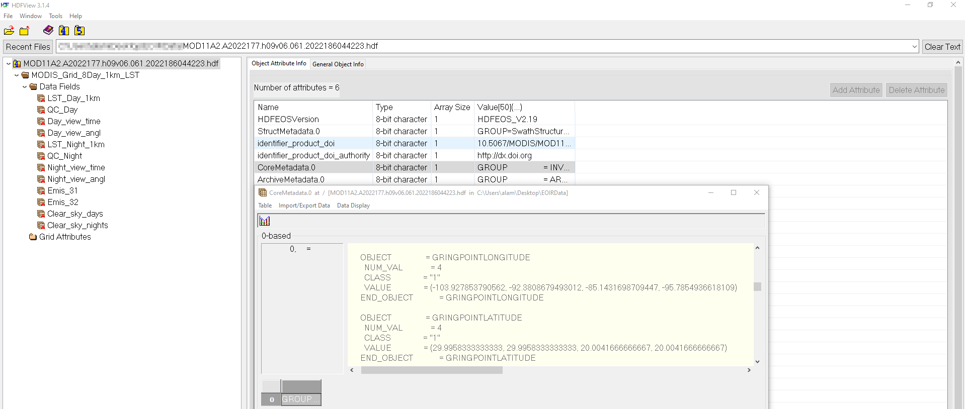
2. Open HDFView and go to File -> Open to load your HDF4 file. In the top-level directory of the file, in the Object Attribute Info tab, locate the the metadata describing the corner lat/lon coordinates of the data. In the MOD11A2 file, this data is located in the CoreMetadata.0 attribute's GRINGPOINTLONGITUDE and GRINGPOINTLATITUDE objects. Make note of these values for later. The lat/lon points in the value array correspond to each other to form a bounding box.
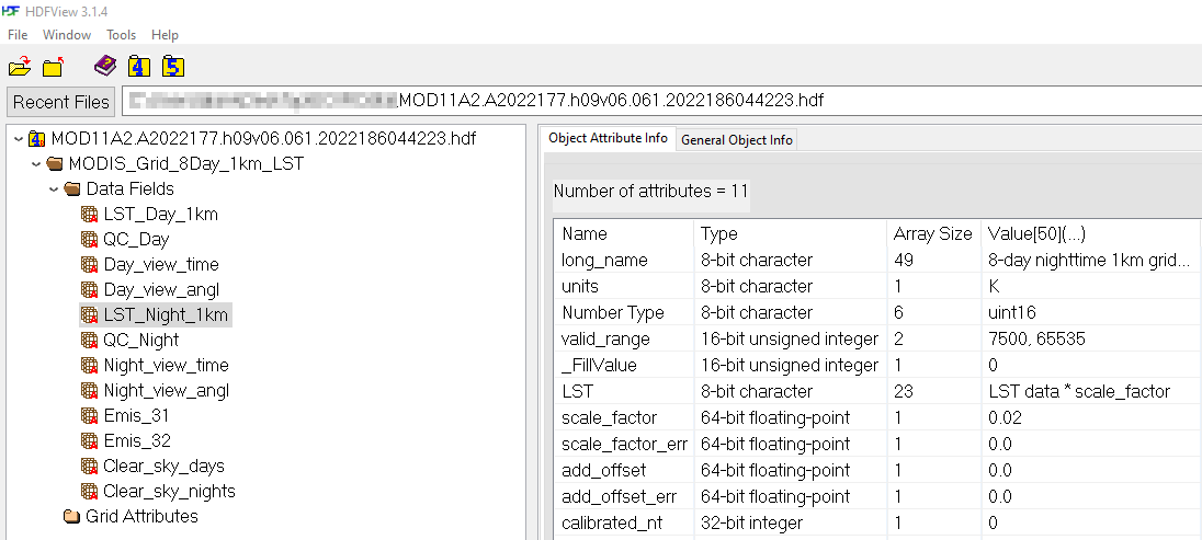
3. Next, in the Data Fields section, locate the desired data set. Note the units, fill value, scale factor, and add offset. In the LST_Night_1km dataset, the units are in Kelvin, which is consistent with STK's expected inputs. In order to convert the data to the true measured land surface temperature, you must multiply the data by a scale factor of 0.02. Sometimes an add offset is also required, but no offset is specified.
4. Save the data so that you can process it properly in Excel. Switch to the General Object Info tab and select the Show Data with Options button. Accept the defaults and click OK. A table with data values will appear; save it by selecting Import/Export Data -> Export Data To -> Text File and saving it to a directory of your choice.
5. You now must import the data into Excel to apply the scaling factor. Open Microsoft Excel, browse to your text file save directory using File -> Open and select your text file. You may need to change the file filter to All Files (*.*) in order to see it. Excel may give you a warning that the file format and extension of the file don't match. You can safely ignore the warning and click Yes to open anyway. The text import wizard will appear, and it has already automatically parsed the contents of your tab-separated text file. Click finish to accept the defaults and import the data.
6. Create a new sheet in the Excel workbook and enter the scaling factor (in this case, it is 0.02) in the first cell. Type Ctrl+C to copy the number in the cell. Then return to the original sheet with data, type Ctrl+A to select the whole sheet. Then right-click and select Paste Special. Set the Operation to Multiply and click OK. This will multiply your entire dataset by the scaling factor. Repeat this if needed using the add operation instead for the add offset, if necessary. If you would like to place a different value instead of the default fill value, you can do so here as well.
7. You are now ready to save the datasheet into a CSV file that STK can read. With the data sheet selected, go to File -> Save As and make sure to save as type CSV UTF-8 (Comma delimited) (*.csv). Excel may give a warning that the selected file type does not support workbooks that contain multiple sheets. Simply click OK to save the active datasheet.
8. You can now load this CSV into STK! Expose the EOIR toolbar by going to View -> Toolbars -> EOIR. Select the EOIR Configuration button -> Atmosphere and Textures button, and select the Texture Maps section. You can now load your texture map by switching 'Value:' to 'File:.' Specify the corner points that you noted earlier. Happy imaging!

HDF5 (*.h5) processing

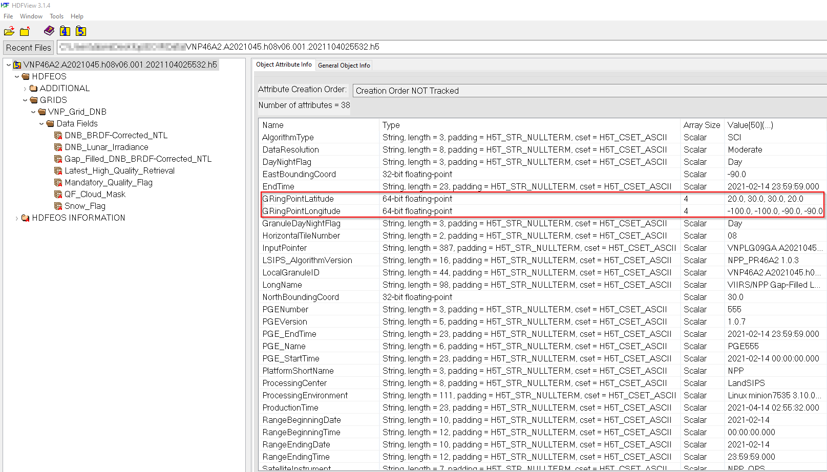
The workflow for processing HDF5 data is largely the same as for HDF4, except that the metadata and data are generally located in a different file structure. Follow the steps for HDF4 processing, except that in step 2, search the Object Attribute Info for the same GRingPointLongitude and GRingPointLatitude objects.


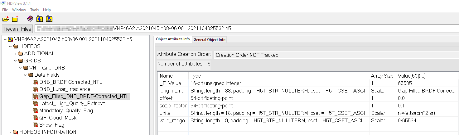
For this specific dataset, when looking at your desired Gap_Filled_DNB_BRDF-Corrected_NTL dataset, you can see that the units are in nWatts/(cm^2 sr) with a scale factor of 0.1 and offset of 0. Also note the fill value of 65535.


You need to convert this radiance value into spectral radiance of units Watts/(cm^2 sr um), which is what STK accepts as an input. In order to do this, you need to know the bandwidth of the sensor used to collect this data. The VIIRS DNB (Day-Night Band) sensor has a bandwidth of 0.4 um according to the sensor suite documentation. So multiplying the data by the scaling factor of 0.1, multiplying by 1E+9 to convert from nWatts to Watts, and then diving by 0.4 to convert radiance to spectral radiance convert the data into the proper units of spectral radiance for STK. Complete this in step 6 above using a factor of 2.5E-10. From the same documentation, the band edges are 0.5 um and 0.9 um. Make note of this for later when specifying the wavelength edges in STK in step 8.

All other steps remain the same as HDF4.

MATLAB

Example processing scripts are available at the AGI Github here. For a general workflow overview, read on below.

HDF4 (*.hdf) processing

1. Use the hdfinfo function to get the metadata from the file. Specifically, locate the metadata containing the corner lat/lon points of the data in the GRingPointLongitude and GRingPointLatitude objects. For the MOD11A2 dataset, you can find this in the CoreMetadata.0 attribute.
2. Browse to the specific scientific dataset (SDS) in question. Here, you are looking for the LST_Night_1km dataset. Get the specific attributes out for that dataset, including scale factor and add offsets.
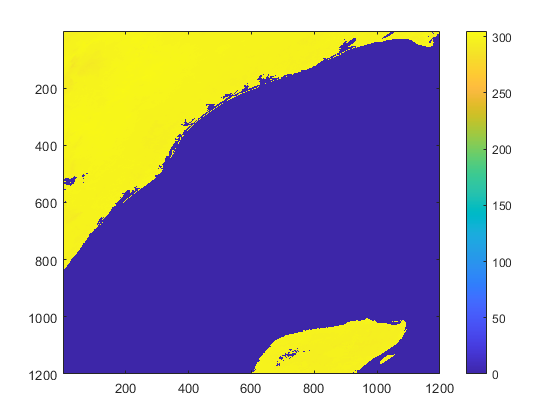
3. Read the data using the hdfread function and apply the scaling factor of 0.02.
4. (Optional) Display the data using the imagesc function. Your image may look very uniform because the fill value creates a large range even though the majority of data has a much smaller range.
5. Write the data to a CSV file using the writematrix function.
6. You can now load this CSV into STK! Expose the EOIR toolbar by going to View -> Toolbars -> EOIR. Select the EOIR Configuration button -> Atmosphere and Textures button and select the Texture Maps section. You can now load your texture map by switching 'Value:' to 'File:.' Specify the corner points that you noted earlier. Happy imaging!

HDF5 (*.h5) processing

1. Use the h5disp function to get the metadata from the file. Specifically, locate the metadata containing the corner lat/lon points of the data in the GRingPointLongitude and GRingPointLatitude. For the VNP46A2 dataset, you can find this in the "/" attributes.
2. Browse to the specific scientific dataset (SDS) in question. You are looking for the Gap_Filled_DNB_BRDF-Corrected_NTL dataset. You can see that the path is /HDFEOS/GRIDS/VNP_Grid_DNB/Data Fields/Gap_Filled_DNB_BRDF-Corrected_NTL. Note the scale factor, units, and offset.
3. Read the data using the h5read function, transpose it, and apply a factor of 2.5e-10. This is to apply the scaling factor, convert nW to W, and then divide by the VIIRS DNB bandwidth of 0.4 um to convert radiance in units nW/(cm^2 sr) to spectral radiance in units W/(cm^2 sr um), which STK will accept. Make a note that the band edges are 0.5 um and 0.9 um. You will need this enter the processed file into STK.
   1. Important: You must transpose all HDF5 data in order to read it properly. This is because MATLAB uses column-major (Fortran-style) order when reading, while the HDF5 standard uses row-major (C-style) order. Transposing the data corrects this difference in reading data.
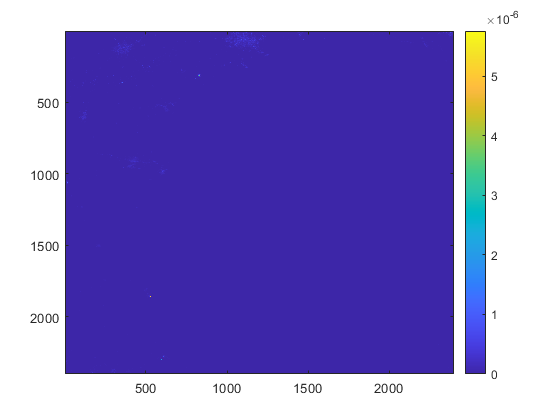
4. (Optional) Display the data using the imagesc function. Your image may look very uniform because the fill value creates a large range, even though the majority of data has a much smaller range.
5. Write the data to a CSV file using the writematrix function.
6. You can now load this CSV into STK! Expose the EOIR toolbar by going to View -> Toolbars -> EOIR. Select the EOIR Configuration button -> Atmosphere and Textures button, and select the Texture Maps section. You can now load your texture map by switching 'Value:' to 'File:.' Specify the corner points that you noted earlier. Happy imaging!

Python

Example processing scripts are available at the AGI Github here. At a minimum, you will need numpy to write data to a file and a package specific to the desired HDF version. For HDF4, you will need pyhdf, and for HDF5, you will need h5py. Matplotlib is optional for inline visualization of your data. Read on for a general overview of the workflow.

HDF4 (*.hdf) processing

Check out the full documentation for pyhdf here.

1. Open the file using pyhdf. Use the .attributes() method to get the file's metadata for the corner points. This is called out by the GRingPointLongitude and GRingPointLatitude objects. You can also use the .datasets() method to get all the datasets available in the file.
2. Use the .select() method to select your desired dataset. For MOD11A2, select LST_Night_1km. Print the attributes to get the dataset-specific attributes like units, fill value, scale factor, and offset.
3. Get the data using the .get() method and apply the scaling factor of 0.02.
4. Write the file to a CSV using numpy's .savetxt method with a comma delimiter. Use the format "%1g" to minimize the size of the file.
5. (Optional) Display the data using matplotlib's imshow method. Your image may look very uniform because the fill value creates a large range even though the majority of data has a much smaller range.
6. You can now load this CSV into STK! Expose the EOIR toolbar by going to View -> Toolbars -> EOIR. Select the EOIR Configuration button -> Atmosphere and Textures button, and select the Texture Maps section. You can now load your texture map by switching 'Value:' to 'File:.' Specify the corner points that you noted earlier. Happy imaging!

HDF5 (*.h5) processing

Check out the full documentation for h5py here.

1. Open the file using h5py. All metadata are arranged as key-value pairs in an H5 file. Print attrs.keys() to see all of the keys associated with the metadata of the file. To index a specific key-value pair, index attrs like a dictionary with square brackets. You can use this method to get the corner points of the data called out by the keys GRingPointLongitude and GRingPointLatitude.
2. Continue using the .keys() method to indexing down to the desired dataset. For VNP46A2, the night light data is located at ['HDFEOS']['GRIDS']['VNP_Grid_DNB']['Data Fields']['Gap_Filled_DNB_BRDF-Corrected_NTL']. Once again, use .attrs.keys() to see dataset-specific metadata, including units, fill value, scale factor, and offset.
3. Read the data by passing the key directly. Then correct your fill value if you desire, and apply a factor of 2.5e-10. This is to apply the scaling factor, convert nW to W, and then divide by the VIIRS DNB bandwidth of 0.4 um to convert radiance in units nW/(cm^2 sr) to spectral radiance in units W/(cm^2 sr um), which STK will accept. Make a note that the band edges are 0.5 um and 0.9 um. You will need this when you enter the processed file into STK.
4. Write the file to a CSV using numpy's .savetxt method with a comma delimiter. Use the format "%1g" to minimize the size of the file.
5. (Optional) Display the data using matplotlib's imshow method. Your image may look very uniform because the fill value creates a large range even though the majority of data has a much smaller range.
6. You can now load this CSV into STK! Expose the EOIR toolbar by going to View -> Toolbars -> EOIR. Select the EOIR Configuration button -> Atmosphere and Textures button, and select the Texture Maps section. You can now load your texture map by switching 'Value:' to 'File:.' Specify the corner points and band wavelengths that you noted earlier. Happy imaging!

General Notes

• Some datasets will not have metadata fields called GRingPointLatitude and GRingPointLongitude to define a bounding box. Instead, a separate data field may include the exact lat/lon points of each pixel. It is up to you to parse the lat/lon data in the same manner as above and to define your own bounding box. Do not use the metadata fields called NorthBoundingCoord, EastBoundingCoord, WestBoundingCoord, or SouthBoundingCoord. These define the extremes of the data and will not be accurate unless the data is arranged north-up in a rectangle.