To design this in the Ansys Systems Tool Kit® (STK®) application, you need to start with a realistic repeat-ground-track-orbit satellite with a realistic area-to-mass ratio. The reason this process works is it uses the atmospheric drag to its advantage by overcorrecting and allowing the drag to restore the orbit.
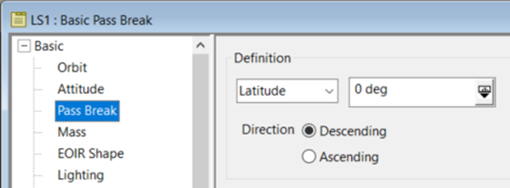
The example satellite in this article is Landsat 7, a near-frozen, sun-synchronous, repeat-ground-track-orbit satellite. It was traditionally analyzed (arbitrarily) using the descending node for passes, and that is what is done in this example. To do this, set it in the satellite's properties under Basic > Pass Break:
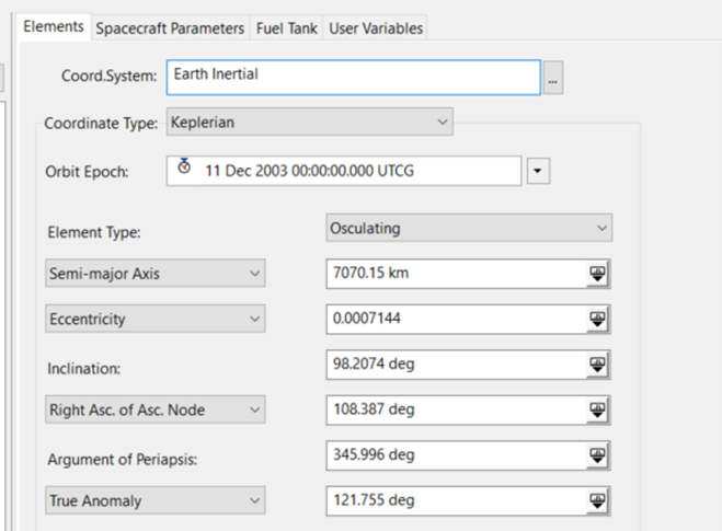
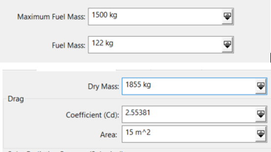
The properties of the satellite are as follows:
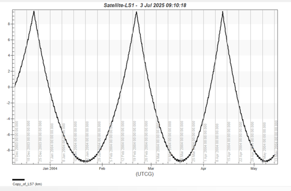
The main analysis is centered around the pass behavior at the equator. The position difference in each pass, the ground track error, is what will drive the correction. The behavior needs to be analyzed visually first.
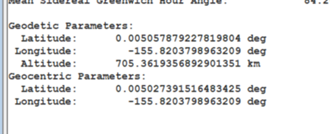
Propagate the satellite to stop at the first descending node and run a segment summary to get the longitude of the descending node it stopped at. You will use this as a reference point.
To support the STK/Astrogator® capability, the Component Browser has Astrogator components. Expand the Calculation Objects folder and select the Ground Track folder. There is one built-in component called RepeatingGroundTrackEquatorError. This calculation object takes in a reference longitude point (the reference descending node just found) and the number of revolutions needed until the ground track repeats, and it calculates the error between sequential descending node passes.
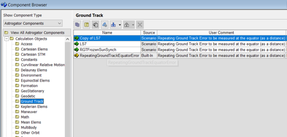
Make a copy of this object using the "Duplicate component" icon, name it LS7, and double-click it to open its properties. Enter the longitude from the segment summary into the ReferenceLongitude row; it will convert to a positive angle direction if it is negative. For Repeat Count, enter the number of revolutions until the ground track repeats. For LS7, this number is 233. Click OK to close the dialog box and save these updates.
Go back to the Basic > Orbit properties of the satellite. Select the Propagate segment and enter 200 for the Repeat Count parameter of the descending node stopping conditions.
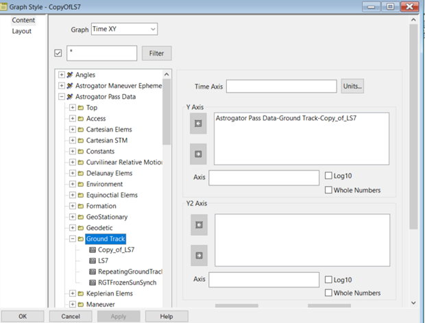
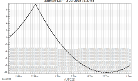
Create a graph using this calculation object, as shown below.
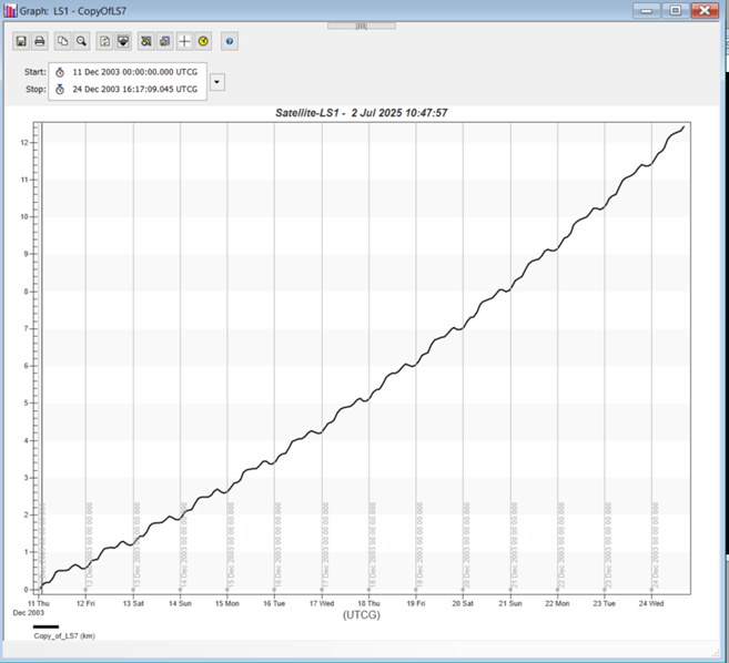
This graph shows that after 200 descending node passes, there is a little over 12 km of ground track error. The next step is to adjust the stopping condition until it stops around where the defined maximum acceptable error is. This example uses 10 km. You can apply a constraint to the descending node stopping condition of the Propagate segment properties. Under Constraints, click the ellipsis next to the text box. The Select Constraints dialog box will appear.

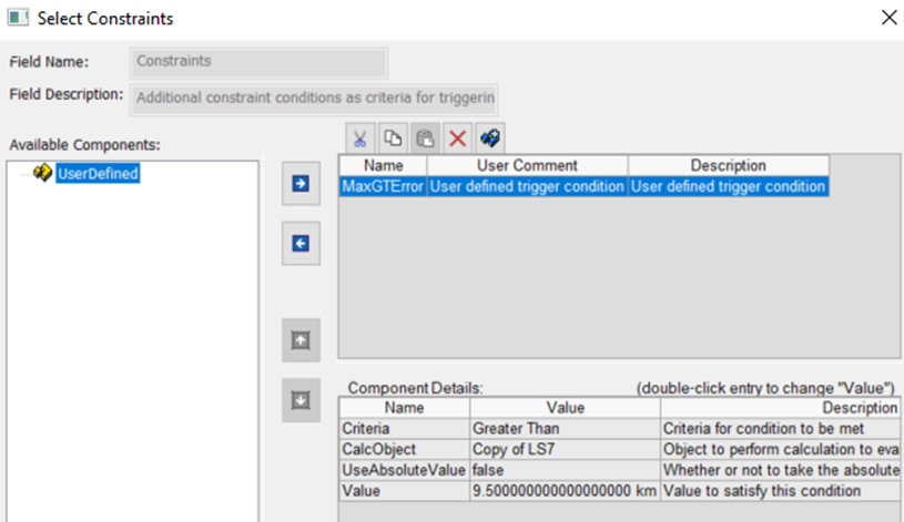
In the dialog box, set CalcObject to the one you created (LS7) in the Component Browser for the ground track error. Set the value to a little bit less than the maximum error. Rename it to something like MaxGTError and set the criteria to Greater Than. This will constrain the stopping condition at the descending node to stop once the ground track error is larger than the specified error. Click OK to save your changes and close the Select Constraints dialog box.
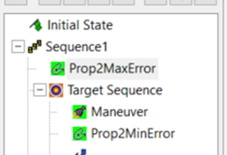
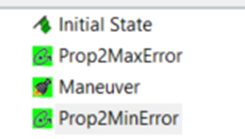
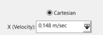
Back in the Astrogator Propagate segment, set Repeat Count back to 1 and run the MCS. The error plot will show the satellite propagating until the error reaches the max error constraint. To correct this, you must insert a maneuver, an impulsive burn in the velocity direction, to adjust the semimajor axis, and therefore the orbit period, slightly. Start with a small burn like 0.1 m/s. Then add another propagate segment after the maneuver to propagate to the 600th descending node, or some other large number, to allow yourself to visually see the behavior.
Refreshing the graph shows that the maneuver was not large enough to bring down the error to the minimum error, which for this exercise is -10 km.
Notice the minimum turnaround, which is the effect of the atmospheric drag pulling the ground track back into the positive error direction. The goal here is to overcorrect the ground track such that atmospheric drag acts to restore it back to the maximum before another burn is performed. This process of propagating to the maximum error and performing a burn to push the ground track to a minimum error, repeats in an oscillatory way when set up correctly, and the atmospheric drag almost acts like another maneuver. The example here is designed to have the ground track within plus or minus 10 km, so the maneuver should push the ground track to around a minimum of -10 km. The point of this part of the exercise is to act like the targeter, changing the thrust in the velocity direction until you see the behavior you want. By trail and error, you end up with the following:
Now that you have a good first guess, the targeter can get a more precise answer. To distinguish when the turnaround point occurs, you can put a constraint onto the Propagate segment that propagates to the minimum error.
If you zoom into the minimum of the graph, you will notice how wiggly the behavior is, so you have to use a method to really ensure when the minimum occurs and when it turns around.
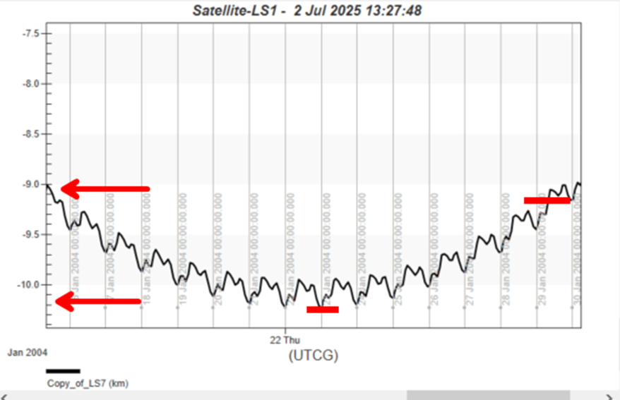
Find a point in the graph where you are sure the curve has risen and has passed the minimum. In this exercise, it is about 1 km above the minimum that you can use as a point in the curve as an indicator that the ground track error is rising again.
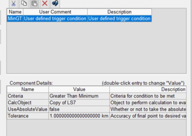
Add a constraint to the propagate segment that uses the ground track error calculation object and the "greater than the minimum" criterion, which is looking for a point in the graph above that is 1 km above the very minimum point. Set the tolerance to 1 km.
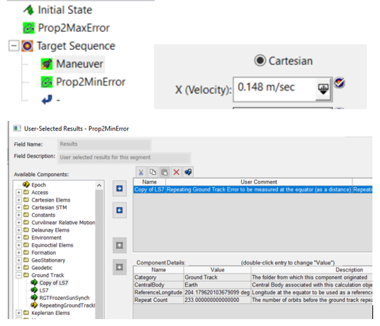
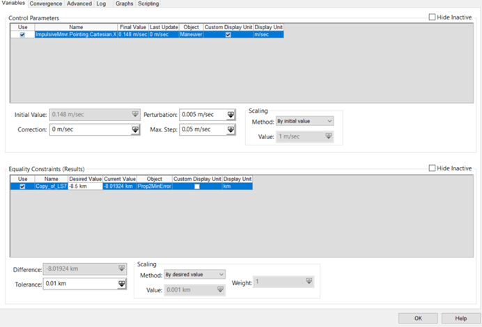
Put the maneuver and the Propagate segment into a targeter. Target the X thrust direction and set the propagate segment result to be the ground track error.
Configure the differential corrector to have the control parameter taking a max step of about 0.05 m/s, with a perturbation of about 0.005. These needed to be adjusted to accommodate the magnitude of the actual maneuver being performed.
Since there was some tolerance of about 0.5 km applied to the maximum error stopping condition (it stopped at +9.5 km error), there will be some applied here too. So you want the minimum to be about -9.5 km; however, since this Propagate segment is actually stopping above the minimum at a point where it is surely rising, the differential corrector actually needs to solve for a position at this tolerance set in the propagate stopping condition constraint. So the desired value is -8.5 km, which is 1 km above the minimum we want of -9.5 km. Set the tolerance to be 0.001.
As a good rule of thumb, it's best to run the targeter once to make sure you set it up correctly. Once that is confirmed, run the targeter and refresh the graph:
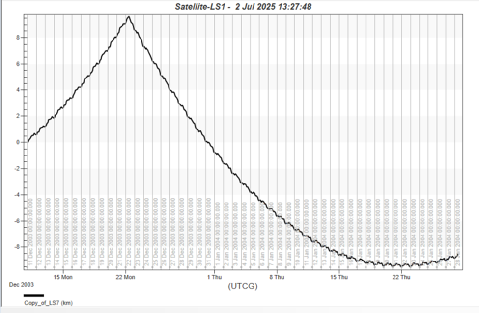
This graph shows correct behavior. You can put this whole thing into a sequence and run it multiple times: